
Fiber links rarely fail loudly. A span that passed acceptance two years ago starts throwing intermittent errors, and the loss budget that looked comfortable on paper no longer closes. Finding the cause means knowing not just that a link is bad, but where along tens of kilometres it went bad. The optical time domain reflectometer, or OTDR, answers that question from one end of the fiber, and no other common field tool returns a distance-resolved picture. The physics behind every OTDR Solution on the market is identical.
An OTDR works by firing a short, high-power pulse of light into one end of a fiber, then measuring how long the returning light took and how strong it is. Because light travels through glass at a known speed, delay converts into distance; because the light is attenuated on both the outbound and return path, the change in strength converts into loss. Plotting strength against distance produces the trace, a curve on which every connector, splice, bend and break appears at its own position.
The chain is easier to follow in the order the light travels.
What Happens Inside an OTDR During a Single Test?
A single test is a four-stage loop: launch a pulse, collect the returning light, convert arrival time into distance, and average many launches into one clean trace. Everything else the instrument reports is derived from that loop.
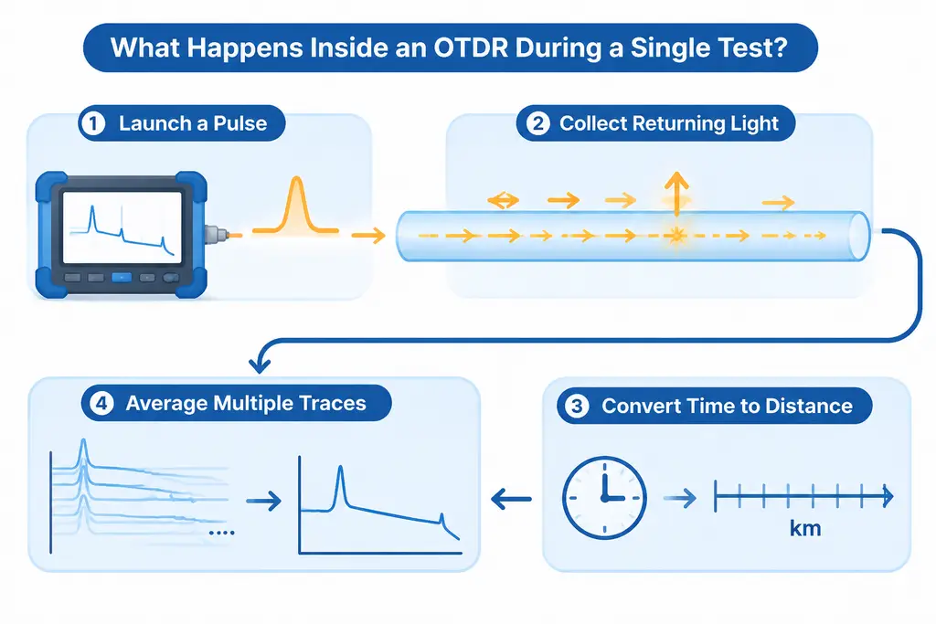
- A laser diode is driven with a short electrical pulse, from a few nanoseconds to a few microseconds wide, and the optical pulse enters the fiber through a coupler.
- As the pulse propagates, a small fraction of its energy scatters backwards off the glass, and larger reflections return from any point where the refractive index changes abruptly.
- An avalanche photodiode converts the returning power into an electrical signal while a clock records the elapsed time of each sample.
- The instrument repeats the launch hundreds or thousands of times and averages the results, because the backscattered signal sits close to the noise floor.
The radar comparison is fair but incomplete. Radar sees discrete targets; an OTDR also reads the continuous weak return from the glass between them, so the trace describes every metre of the path.
Because the pulse leaves and returns through the same port, one technician can characterise a link tens of kilometres long, which is why the OTDR dominates acceptance testing and fault location.
Two Kinds of Return Light Explain the Whole Trace
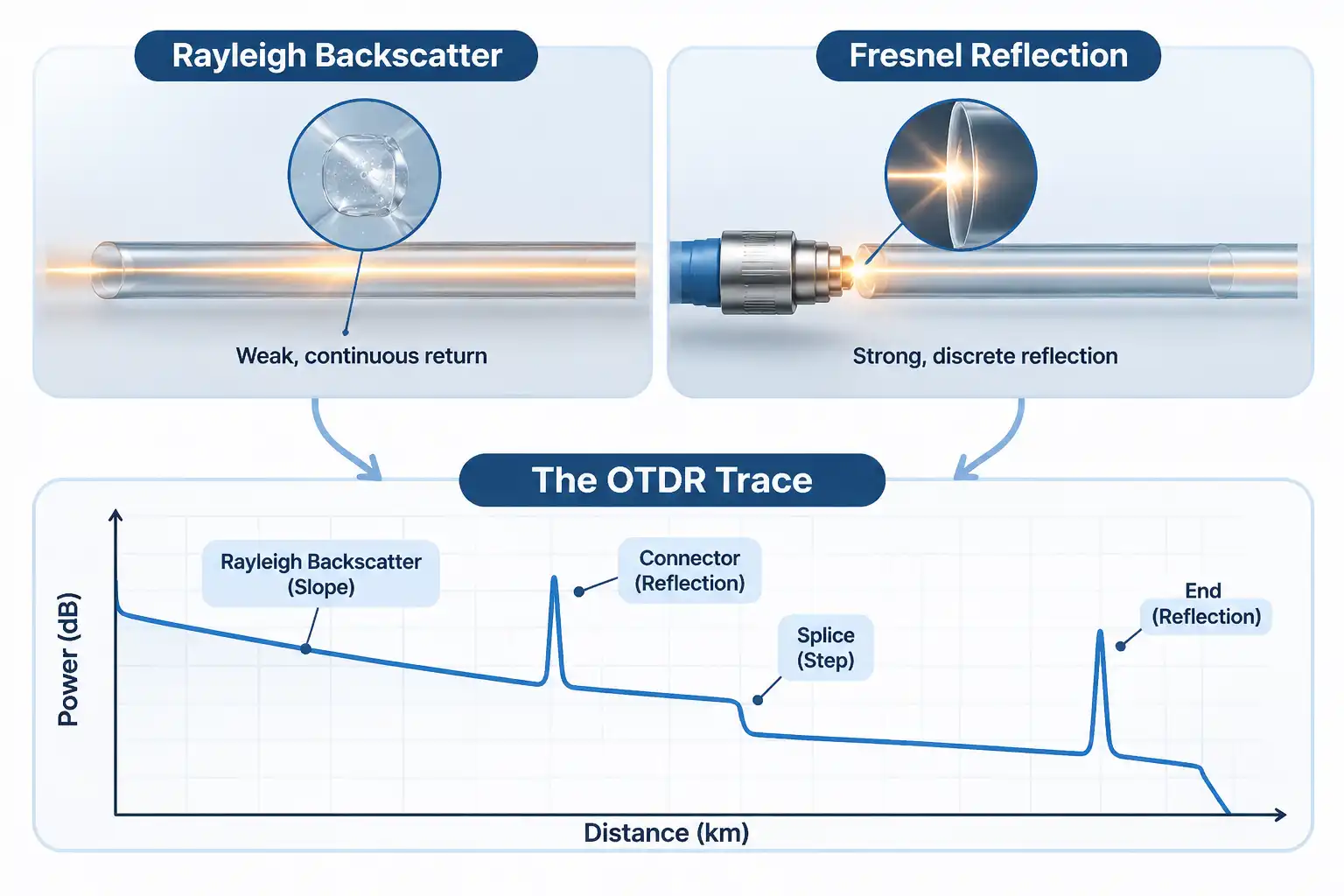
The trace is built from two physically different returns: Rayleigh backscatter, a weak continuous signal from the glass itself, and Fresnel reflection, a strong discrete signal from abrupt changes in refractive index. The first gives the slope, the second gives the events.
Rayleigh backscatter as the continuous baseline
Rayleigh scattering occurs because glass is not optically perfect at the microscopic level. Density fluctuations scatter a small part of the travelling pulse, and a tiny, pulse-width-dependent fraction of the launched energy comes straight back — typically 75 to 80 dB below launch per meter of pulse width. That figure is tiny, so averaging is mandatory, but it is stable, which is why the slope is meaningful. Because scattered power falls on both the outbound and return path the trace slopes downward, and shorter wavelengths scatter more strongly, so a 1310 nm trace sits above a 1550 nm trace.
Fresnel reflection as the discrete event marker
Wherever the pulse meets a step change in refractive index, part of it reflects back coherently instead of scattering. A cleaved end, a connector air gap, a mechanical splice or a break all produce such a step, and the reflection can be 30 dB or more above the backscatter level, hence the spike. A fusion splice, where two fibers are welded into one piece of glass, produces almost no reflection and shows only a small step down.
Where the three “C”s of fiber show up in the trace
The three ”C“s of fiber, core, cladding and coating, describe the construction the trace reports on. The core carries the light and sets the backscatter baseline; the cladding confines it through the index step at its boundary; the coating strips escaped light, so a tight bend shows up as loss at the longer test wavelengths.
How Does the OTDR Convert Time Into Distance and dB?
Distance comes from the round-trip delay of each sample, corrected for the speed of light in that fiber. Loss comes from the difference in power level between two points on the trace.
The round-trip time formula
The conversion is d = c x t / (2 x IOR), where c is the speed of light in vacuum, t is the round-trip time, IOR is the group index of the fiber, and the factor of two accounts for the light travelling out and back. Single-mode fiber at 1550 nm has an index near 1.468, so light covers about 1 m in 5 ns, and an event 1 m away returns after roughly 10 ns. If the index is wrong, every distance is wrong by the same proportion, which is why the datasheet value must be entered rather than a default. Field accuracy is typically plus or minus 1 m plus a small percentage of distance. ITU-T G.650.3 defines the standard test methods for installed single-mode fiber links.
Reading attenuation coefficient from the slope
Two markers placed on a clean stretch of trace away from any event give a distance and a power difference, and the ratio is the attenuation coefficient in dB/km. Typical single-mode values are about 0.35 dB/km at 1310 nm and 0.20 to 0.25 dB/km at 1550 nm. A marker on the curved recovery region beside a reflective event inflates the reading, so most instruments offer a least-squares fit across the segment.
How Do You Read an OTDR Trace Event by Event?
Each type of event has a recognisable signature, so a trace is read by shape first and by number second. A spike means reflection, a step means loss, and a step with a spike means both.
| Event | Trace signature |
| Connector | Sharp reflection spike followed by a step down |
| Fusion splice | Small step down, no spike |
| Macro-bend or kink | Loss step with little or no reflection |
| Break | Large reflection or abrupt drop into noise |
| Fiber end | Strong terminal spike, then noise floor |
| Splitter | Symmetrical step, one per output branch |
Ghosts and gainers, the two artifacts that mislead
A ghost is a reflection that reappears where nothing physical exists, created when a strong reflection bounces back to the launch connector and travels out again. Ghosts sit at predictable multiples of real event distances and carry no loss of their own, so an event with zero loss and a symmetrical twin is almost always a ghost. A gainer is the opposite: a splice that appears to add light. The cause is a difference in backscatter coefficient between two fibers, not amplification, and averaging both test directions removes it.
Why Do Pulse Width, Dead Zone and Dynamic Range Pull Against Each Other?
A wider pulse carries more energy, so it reaches further and produces a larger dynamic range, but it also blinds the receiver for longer after every reflection, which widens the dead zone. Narrow pulses give detail near the instrument, wide pulses give reach at the far end.
The event dead zone is the minimum spacing at which two reflective events can still be distinguished, and it is set almost entirely by pulse width. The attenuation dead zone is longer: the distance after a reflection before loss can be read accurately again. Short-pulse single-mode instruments commonly specify event dead zones of 1 to 3 m, with attenuation dead zones several times that. Dead zone and dynamic range figures are only comparable at the same pulse width, which is why a datasheet for a field OTDR System lists several pulse settings rather than one headline number.
| Pulse width | Behaviour | Typical use |
| 3 to 10 ns | Smallest dead zone, least reach | Patch panels, data centre links |
| 30 to 100 ns | Balanced | Metro and access spans |
| 1 to 20 us | Largest dynamic range, widest dead zone | Long haul and submarine spans |
Longer averaging lowers the noise floor and increases usable dynamic range, by roughly 1.5 dB per doubling of averaging time — about 2.4 dB from one minute to three; beyond about ten minutes the improvement flattens out. Both wider pulses and longer averaging buy reach, but only the first costs resolution.
What Are the Four Parameters of an OTDR Setup?
The four parameters that define a test are wavelength, pulse width, range and averaging time, with the index of refraction and the event threshold as supporting settings. Wavelength decides what the test is sensitive to, pulse width decides resolution against reach, range decides the sampling window, and averaging decides how far into the noise you can see.
| Parameter | Setting rule | Common mistake |
| Wavelength | Match the service band and test at two | A single wavelength hides bend loss |
| Pulse width | Shortest that still reaches the far end | One wide pulse for a whole link |
| Range | 1.5 to 2 times the fiber length | Range shorter than the link, truncating the end |
| Averaging time | 30 s to 3 min for field work | Assuming longer is always better |
The index of refraction scales every distance on the trace, and the event threshold decides which small steps are reported at all. A threshold set above a good splice loss will hide that splice completely. The Fiber Optic Association publishes a field procedure for OTDR measurement covering marker placement for length, attenuation, splice loss and reflectance.
Can You Test Live Fiber With an OTDR?
Yes, but only with an instrument and a port designed for it. A standard 1310 or 1550 nm port must never be connected to a fiber carrying traffic, because the test pulse would travel into the live path while the downstream signal swamps or damages the receiver. In-service testing uses the maintenance band at 1625 or 1650 nm through a filtered port that blocks the traffic wavelengths.
The filter is the part that is easy to overlook. A port that emits 1625 nm is not automatically safe; it becomes safe when the receiver is protected from the 1310, 1490 and 1550 nm light already on the fiber.
The longer maintenance wavelength brings a second benefit. Bend loss grows with wavelength, so 1625 and 1650 nm expose the tight bends at wall boxes and in cabinets well before those bends affect the traffic band. Before connecting anything, measure the received power at the subscriber end: if it is normal, the fault is more likely in the terminal equipment than in the fiber. Continuous versions of this approach are described in the network monitoring solution overview, where tests at the maintenance wavelength run without touching live service.
How Does the Working Principle Scale to Continuous Monitoring?
The principle does not change when the test becomes automatic. What changes is that a stored reference trace replaces the technician’s judgement, and every later trace is compared against it, so a shift of a few tenths of a dB at a known distance is enough to raise an alarm before the link fails.
A launch cable of sufficient length, typically 100 m or more on single-mode outside plant, keeps the first connector out of the dead zone and lets the instrument recover from its own initial pulse; a receive cable does the same for the last connector. Bidirectional testing, with the two results averaged, then removes the direction-dependent error that makes a splice look like a gainer from one side.
Scale that up and a remote test unit behind an optical switch can poll dozens of fibers on a schedule, storing baselines and comparing them automatically. The same backscatter physics also underpins distributed sensing, where the fiber becomes the sensor rather than the object under test, as in DAS Distributed Acoustic Sensing. In every case the instrument is doing what it did on the first day: sending a pulse, timing what returns, and turning delay into distance.
FAQ
Three questions come up repeatedly once the measurement chain is understood.
Does an OTDR replace an insertion loss test?
No. An insertion loss test with a source and power meter measures total end-to-end loss in the direction traffic travels, and it remains the reference for whether a link meets its loss budget. An OTDR adds per-event detail that a total loss figure cannot show, but it is not a substitute for the loss measurement.
Can an OTDR see through a PON splitter?
Only with enough dynamic range and the right test mode. Each doubling of split ratio costs roughly 3 dB, so a 1:32 splitter costs at least 15 dB of theoretical splitting loss — typically 17 to 18 dB of insertion loss in practice before any fiber loss is counted.A high dynamic range instrument with a dedicated splitter mode can measure beyond one splitter stage, though reflections from other branches complicate the trace.
How often does an OTDR need calibration?
Most manufacturers recommend annual calibration to keep loss and distance accuracy inside specification. Day-to-day reliability depends far more on connector care: a contaminated end face on the test port creates artificial reflectance, widens the dead zone and corrupts every measurement taken through it.