
Pipeline operators, perimeter security teams, and rail asset managers all have to justify monitoring decisions with numbers, and few numbers are as widely quoted and as widely misunderstood as the sensitivity of distributed acoustic sensing. A single cable buried beside a pipeline can act as thousands of acoustic sensors at once, which looks convincing on paper. The difficulty starts when procurement asks what the system can actually detect, because the answer is usually one figure with no context attached.
Distributed acoustic sensing typically resolves strain changes in the picostrain to low nanostrain range: a well-designed interrogator reaches a noise floor of roughly 1 to 30 pε/√Hz at an 8 m gauge length near 100 Hz, equivalent to phase noise of about 70 μrad/√Hz to 2 mrad/√Hz. That figure is not a constant. It varies by more than an order of magnitude with gauge length, acoustic frequency, position along the fiber, cable construction, and the optical architecture of the interrogator.
The factors behind that spread are well understood, and each one can be engineered around.
What Sensitivity Means in Distributed Acoustic Sensing
Sensitivity in distributed acoustic sensing is the smallest optical phase change the interrogator can distinguish from its own noise, converted into an equivalent strain over a defined length of fiber and expressed as a spectral density per root-hertz of measurement bandwidth.
The instrument never measures sound pressure directly. What it measures is the time-resolved phase of coherent light that has been Rayleigh-scattered inside the fiber, and that phase is coupled to mechanical strain through the glass. Sensitivity is therefore a statement about phase first and strain second, and the conversion between the two depends on parameters that belong to the fiber and the configuration rather than to the instrument alone.
Recent theoretical work on the transfer function from acoustic pressure to phase has clarified an important detail: the fiber responds to acoustic pressure in the incident wave rather than to radial or axial particle displacement, and the angular and frequency dependence of that response is strongly shaped by resonance scattering from an axially symmetric vibration mode of the fiber. A sensitivity figure measured with a bonded piezoelectric stretcher is therefore not automatically transferable to a buried cable responding to a pressure wave.
Phase Noise Floor Versus Strain Sensitivity
Interrogators are characterised natively in radians, with the noise floor quoted as an amplitude spectral density in rad/√Hz or as dB relative to 1 rad/√Hz. Converting to strain requires the optical wavelength, the group index of the fiber, the gauge length, and a photo-elastic scaling factor. This is why a strain sensitivity quoted without a gauge length and a reference frequency carries almost no information: the same hardware can appear twenty times more or less sensitive depending on how those two numbers are chosen.
Why Sensitivity Is Not the Same as Resolution
Four quantities are routinely confused in datasheets and tender documents, and they answer different questions:
- Minimum detectable strain, the sensitivity figure itself, describing how small a change can be seen.
- Spatial resolution, describing how short an event can be separated from its neighbours along the fiber.
- Spatial sample spacing, describing how densely output channels are produced, which is often finer than the true resolution.
- Location accuracy, describing how precisely an event position can be reported, which depends on sampling, signal-to-noise ratio, and processing.
A system can be extremely sensitive and still unable to separate two events three meters apart.
How Distributed Acoustic Sensing Works
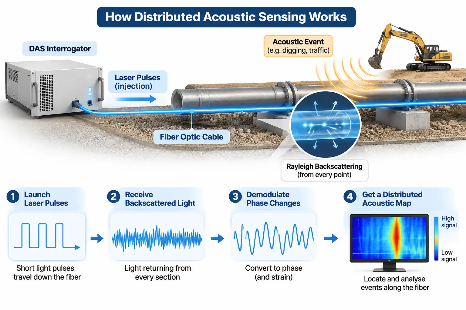
A distributed acoustic sensing interrogator launches coherent laser pulses into a fiber and continuously demodulates the phase of the light that Rayleigh scattering sends back; because return time maps directly to distance, every section of the fiber becomes a virtual acoustic sensor with no transducers in the field.
Each pulse travels down the fiber and a small fraction of its energy is scattered backwards by intrinsic density and refractive-index fluctuations, the same Rayleigh backscattering mechanism that limits loss in any telecom link. Light returning from a section roughly one pulse length long interferes at the receiver, and the resulting phase depends on the optical path length between the scatterers in that section. When the fiber is stretched or compressed, the path length changes and the phase moves with it.
From Backscattered Light to Phase
The measurement architecture is a phase-sensitive optical time-domain reflectometer. A narrow-linewidth source is modulated into pulses, an erbium-doped fiber amplifier sets the launch power, and a coherent receiver mixes the returning field with a local oscillator or an acousto-optic frequency shift. In-phase and quadrature components are sampled at the interrogation rate, and phase is extracted and unwrapped channel by channel. The quality of that demodulation chain, not the fiber, usually decides the noise floor.
Why the Fiber Itself Is the Sensor
A standard single-mode fiber is an intrinsically sensitive strain gauge. Axial strain changes both the physical length of the section and its refractive index through the photo-elastic effect, and the two contributions combine into a scaling factor close to 0.78 for longitudinal strain. Because the sensing element is ordinary glass with no electronics at the measurement point, the approach suits pipelines, tunnels, subsea cables, and other locations where powered sensors are impractical.
Factor 1: Gauge Length and the Sensitivity-Resolution Trade-Off
Gauge length is the length of fiber over which the phase change is integrated, so a longer gauge length accumulates a larger phase shift for the same applied strain and therefore delivers better strain sensitivity, at the cost of spatial detail.
Gauge length settings on current distributed acoustic sensing equipment span roughly 0.8 m to 16 m, and that range alone produces a twenty-fold change in strain sensitivity with no hardware modification. The relationship is simple: the strain equivalent of one radian of phase is inversely proportional to gauge length.
| Gauge length | Strain per radian of phase | Relative strain sensitivity | Practical consequence |
| 0.8 m | about 135 nε/rad | Lowest | Fine spatial detail, weakest weak-signal performance |
| 1.6 m | about 67 nε/rad | Low | Good for short-duration, localized events |
| 3.2 m | about 34 nε/rad | Moderate | Balanced setting for most infrastructure work |
| 8 m | about 13.5 nε/rad | High | Common reference point for published noise floors |
| 16 m | about 6.7 nε/rad | Highest | Best faint-signal detection, blurred short events |
The same averaging that improves sensitivity also acts as a spatial low-pass filter. Strain features shorter than roughly one gauge length are partly cancelled inside the integration window, so a long gauge length can hide a crack-induced transient that a short setting would resolve. Choosing a gauge length is therefore a statement about what the monitoring objective actually is, not a matter of selecting the most sensitive option available.
Factor 2: Frequency Response and the Noise Floor
Sensitivity is strongly frequency dependent: it is poorest at the low end, where drift and thermal effects dominate, is best from roughly 10 Hz to a few kilohertz, and falls again as interrogation rate and pulse energy limit the response.
Low-Frequency Behaviour
Below a few hertz, several noise sources rise together. Laser frequency noise appears directly in the demodulated phase, temperature changes alter both fiber length and refractive index, and installation settlement produces slow apparent strain. The practical floor at 0.1 Hz is usually set by the environment and the cable rather than by the interrogator, which is why low-frequency claims should always be tied to a specific installation.
High-Frequency Limits
Two constraints cap the upper end. The first is temporal: a single pulse must complete its round trip before the next one is launched, so the unambiguous interrogation rate is approximately c/(2nL).
| Fiber length | Maximum unambiguous interrogation rate | Nyquist-limited acoustic bandwidth |
| 10 km | about 10.2 kHz | about 5.1 kHz |
| 25 km | about 4.1 kHz | about 2.0 kHz |
| 50 km | about 2.0 kHz | about 1.0 kHz |
The second constraint is spatial: the gauge length averages the strain field, so acoustic wavelengths approaching twice the gauge length are attenuated in the output. Long reach and high bandwidth pull in opposite directions, and any claim of very wide bandwidth should be checked against the fiber length it was measured on.
Factor 3: Interrogator Architecture
The hardware sets the sensitivity ceiling: laser coherence determines how much usable phase information returns, pulse energy and optical budget determine how far it survives, and the detection scheme determines how much of it can be recovered.
Laser Coherence and Phase Noise
Coherence length must comfortably exceed the round-trip path difference that produces interference at the receiver. A source with insufficient coherence decorrelates the scatterers within a section and washes out the phase signal, while excessive frequency noise converts directly into strain noise at low Fourier frequencies.
Polarization Fading and Diversity Detection
The polarization state of backscattered light drifts along the fiber, and where the returning state becomes orthogonal to the local oscillator the interference contrast collapses. The result is not a uniform loss of sensitivity but localized dead spots that move with temperature. Polarization-diversity receivers remove most of this effect, and its presence or absence explains many gaps between two systems tested on the same cable.
Optical Budget and Sampling
Returned power scales with pulse energy, so the practical ceiling of a DAS System is set by the onset of nonlinear effects in the fiber, the noise figure of the amplifier chain, and the effective resolution of the digitiser. Receiver noise, not signal level, sets the floor once the optical budget is exhausted.
Factor 4: Fiber, Cable and Installation
No interrogator can recover a signal that never reaches the fiber core, so cable construction and installation practice frequently dominate field sensitivity more than any single datasheet parameter.
Strain Transfer and Cable Construction
Loose-tube cables decouple the fiber from the surrounding jacket to protect it from mechanical load, and that same decoupling attenuates acoustic coupling. Tight-buffered designs transfer strain more faithfully but are less forgiving during installation. Gel filling inside a loose tube can improve acoustic coupling to the surrounding medium, but it does not restore axial strain transfer.Jacket stiffness, armouring, and the bedding material between cable and structure all act as mechanical filters with their own frequency response. Fiber design matters too: cladding geometry can shift resonance scattering out of the propagating regime and measurably improve signal-to-noise ratio.
Environmental Noise and Common-Mode Rejection
Most field deployments run inside a wider Optical Fiber Monitoring System that also covers fault location, asset records, and alarm routing. Within that system, the dominant limit is often ambient noise: traffic, pumps, compressors, and wind acting on exposed spans. Because these sources are spatially broad, adjacent channels share them, and differential or array-based processing can recover weak local events that would otherwise stay buried.
Factor 5: Range and Distance
Sensitivity declines with distance because Rayleigh backscatter is attenuated on the way out and on the way back while the receiver noise floor stays fixed, so the same link delivers noticeably better sensitivity at 2 km than at 40 km.
Standard single-mode fiber loses roughly 0.2 dB per kilometer at 1550 nm, and the round trip doubles that, so a 25 km span returns about 10 dB less light than a 2 km span and a 50 km span about 20 dB less. Because signal-to-noise ratio scales with returned power, the noise floor in strain terms rises by an order of magnitude or more across that distance. Long-range designs compensate with higher pulse energy, Raman or discrete amplification, and pulse coding, but none of these removes the trade-off between reach and sensitivity.
How to Calculate and Compare DAS Sensitivity
Convert a quoted phase-noise floor into strain sensitivity with the standard relation, then compare only figures measured at identical gauge length, wavelength, and frequency.
The definition is standardised in IEC 61757-3-2, which relates the phase noise floor to gauge length through a photo-elastic scaling factor of 0.78:
ε_sens = λ · δφ / (4π · n · G · ξ)
where λ is the vacuum wavelength, δφ the phase noise in radians, n the group index of the fiber, G the gauge length, and ξ the photo-elastic factor. At 1550 nm with n ≈ 1.468 and G = 8 m, one radian corresponds to about 13.5 nε, so:
| Quoted noise floor | Phase noise | dB re 1 rad/√Hz | Typical context |
| 1 pε/√Hz | about 74 μrad/√Hz | about −83 dB | Short-range, optimised laboratory-grade settings |
| 5 pε/√Hz | about 0.37 mrad/√Hz | about −69 dB | Standard mid-range operation |
| 30 pε/√Hz | about 2.2 mrad/√Hz | about −53 dB | Long-range unit at 8 m gauge length and 100 Hz |
A practical comparison follows four steps: confirm the gauge length, confirm the reference frequency and bandwidth, check whether the figure is a strain or phase quantity, and verify the fiber length over which it was measured. Any quotation missing one of these four items should be treated as indicative rather than comparable.
Beyond DAS: How DFOS Modalities Compare
Distributed fiber optic sensing turns a fiber into a continuous array by interpreting backscattered light; DAS reads phase for acoustic signals, DVS reads intensity for vibration events, and DTS reads Raman scattering for temperature, each with its own sensitivity metric.
| Modality | Scattering mechanism | Measurand | Sensitivity metric | Typical role |
| DAS | Rayleigh, phase demodulated | Dynamic strain and acoustic pressure | pε/√Hz or rad/√Hz | Acoustic signatures, leak and intrusion detection |
| DVS | Rayleigh, intensity only | Vibration events | Event threshold, not spectral density | Simple perimeter and fence alarm |
| DTS | Raman | Temperature | °C and spatial resolution | Cable thermal monitoring, fire detection |
| Brillouin-based | Brillouin frequency shift | Static strain and temperature | με and °C | Structural deformation monitoring |
Simpler installations often use DVS Distributed Vibration Sensing, which detects and locates vibration events from intensity changes alone. It costs less and needs no phase demodulation, but it cannot reconstruct a waveform or a spectral signature, which is precisely where DAS earns its higher price. The sensitivity of a DAS system should therefore be judged against what the application needs to classify, not against the largest number on a datasheet.
Frequently Asked Questions
Sensitivity questions usually come down to three practical concerns: whether the numbers are physically meaningful, how configuration choices interact, and what cannot be improved simultaneously.
Can distributed acoustic sensing detect sub-nanostrain changes?
Yes, comfortably. A nanostrain is roughly two hundred times the per-root-hertz noise floor of a mid-range system (5 pε/√Hz) at an 8 m gauge length, and even picostrain-level disturbances remain measurable in the middle of the band. The limiting factor in most field installations is not the interrogator but the acoustic coupling between the event and the cable.
Is a shorter gauge length always better for detail?
No. A short gauge length improves spatial resolution but reduces the phase accumulated per unit strain, so weak or distant events become harder to detect. The usual rule is to set the gauge length at or below half the shortest spatial wavelength of interest, then confirm that the resulting signal-to-noise ratio is still adequate for the event class being monitored.
Can sensitivity and dynamic range be improved at the same time?
Rarely, because both compete for the same optical and electronic resources. Raising launch power improves weak-signal detection but pushes the fiber toward nonlinear effects and can saturate strong near-field events, while aggressive amplification adds noise. Practical designs instead segment the fiber into zones with different settings or apply time-varying gain, accepting a compromise rather than maximising either figure.